Artificial Intelligence & Machine Learning 2 - Linear Regression | Stanford CS221: AI (Autumn 2021)

import numpy as np

#######################################
# Optimization problem
trainExamples = [
    (1, 1),
    (2, 3),
    (4, 3),    
]

def phi(x):
    return np.array([1,x])

def initialWeightVector():
    return np.zeros(2)

def trainLoss(w):
    return 1.0 / len(trainExamples) * sum((w.dot(phi(x)) - y)**2 for x, y in trainExamples)

def gradientTrainLoss(w):
    return 1.0 / len(trainExamples) * sum(2 * (w.dot(phi(x)) - y) * phi(x) for x, y in trainExamples)



#######################################
# Optimization algorithm
def gradientDescent(F, gradientF, initialWeightVector):
    w = initialWeightVector()
    eta = 0.1
    for t in range(500):
        value = F(w)
        gradient = gradientF(w)
        w = w - eta * gradient
        print(f'epoch {t}: w = {w}, F(w) = {value}, gradientF = {gradient}')

Artificial Intelligence & Machine learning 3 - Linear Classification | Stanford CS221 (Autumn 2021)

import numpy as np

#######################################
# Optimization problem

trainExamples = [
	# (x, y) pairs
    ((0, 2), 1),
    ((-2, 0), 1),
    ((1, -1), -1),    
]

def phi(x):
    return np.array([x)

def initialWeightVector():
    return np.zeros(2)

def trainLoss(w):
    return 1.0 / len(trainExamples) * sum(max(1 - w.dot(phi(x)) * y, 0) for x, y in trainExamples)

def gradientTrainLoss(w):
    return 1.0 / len(trainExamples) * sum(-phi(x) * y if 1 - w.dot(phi(x)) * y > 0 else 0 for x, y in trainExamples)



#######################################
# Optimization algorithm
def gradientDescent(F, gradientF, initialWeightVector):
    w = initialWeightVector()
    eta = 0.1
    for t in range(500):
        value = F(w)
        gradient = gradientF(w)
        w = w - eta * gradient
        print(f'epoch {t}: w = {w}, F(w) = {value}, gradientF = {gradient}')

 

 

 

 

 

 

import numpy as np
import math

#######################################
#Optimization ptoblem

trueW = np.array([1, 2, 3, 4, 5])
def generate():
    x = np.random.randn(len(trueW))
    y = trueW.dot(x) + np.random.randn()
    print('example', x, y)
    return (x, y)
trainExamples = [generate() for i in range(1000000)]

def phi(x):
    return np.array(x)

def initialWeightVector():
    return np.zeros(len(trueW))

def trainLoss(w):
    return 1.0 / len(trainExamples) * sum((w.dot(phi(x)) - y) ** 2 for x, y in trainExamples)

def gradientTrainLoss(w):
    return 1.0 / len(trainExamples) * sum(2 * (w.dot(phi(x)) - y) * phi(x) for x, y in trainExamples)

def loss(w, i):
    x, t = trainExamples[i]
    return (w.dot(phi(x)) - y)**2

def gradientLoss(w, i):
    x, y = trainExamples[i]
    return 2 * (w.dot(phi(x)) - y) * phi(x)

#######################################
# Optimization algorithm
def stochasticGradientDescent(f, gradientf, n, initialWeightVector):
    w = initialWeightVector()
    numUpdates = 0
    
    for t in range(500):
        for i in range(n):
            value = f(w, i)
            gradient = gradientf(w, i)
            numUpdates += 1
            eta = 1.0 / math.sqrt(numUpdates)
            w = w - eta * gradient
        print(f'epoch {t}: w = {w}, F(w) = {value}, gradientF = {gradient}')

#gradientDescent(trainLoss, gradientTrainLoss, initialWeightVector)
stochasticGradientDescent(loss, gradientLoss, len(trainExample), initialWeightVector)

Artificial Intelligence & Machine Learning 4 - Stochastic Gradient Descent | Stanford CS221 (2021)

Gradient descent의 단점 : slow

why) each literation requires going over all training examples

it's expensive when we have large data

 

solution) Stochastic Gradient Descent

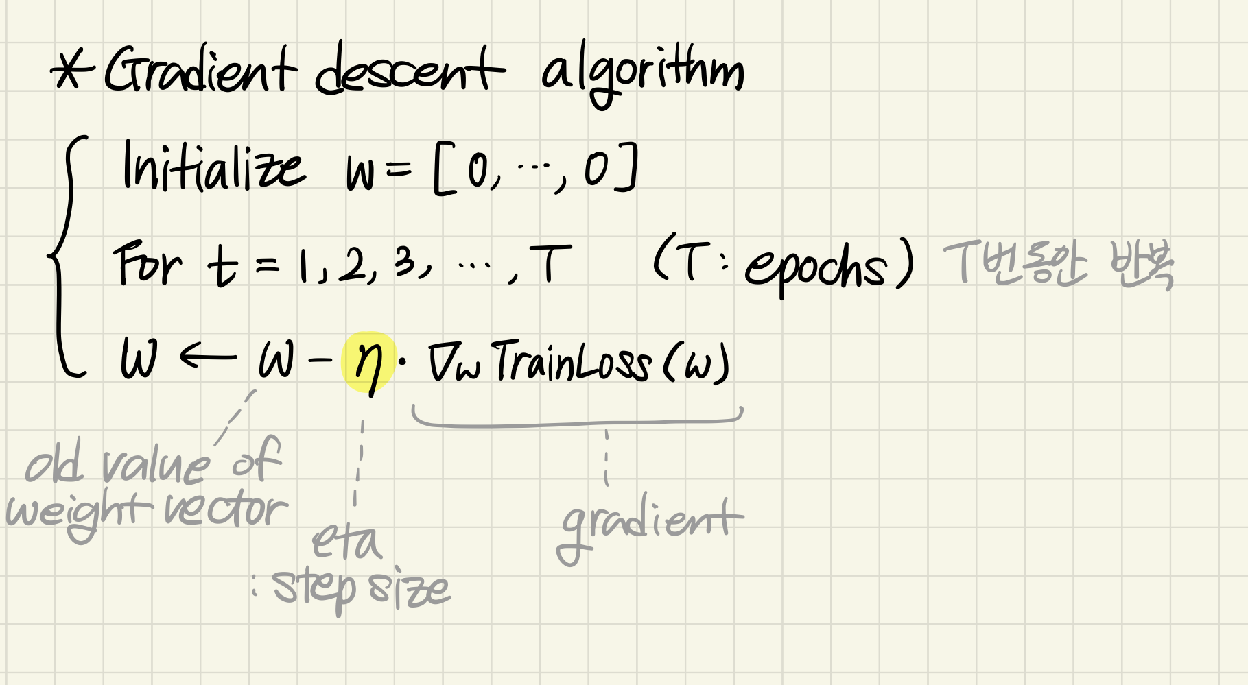
going through the training set and performing one update

 

 

 

 

 

 

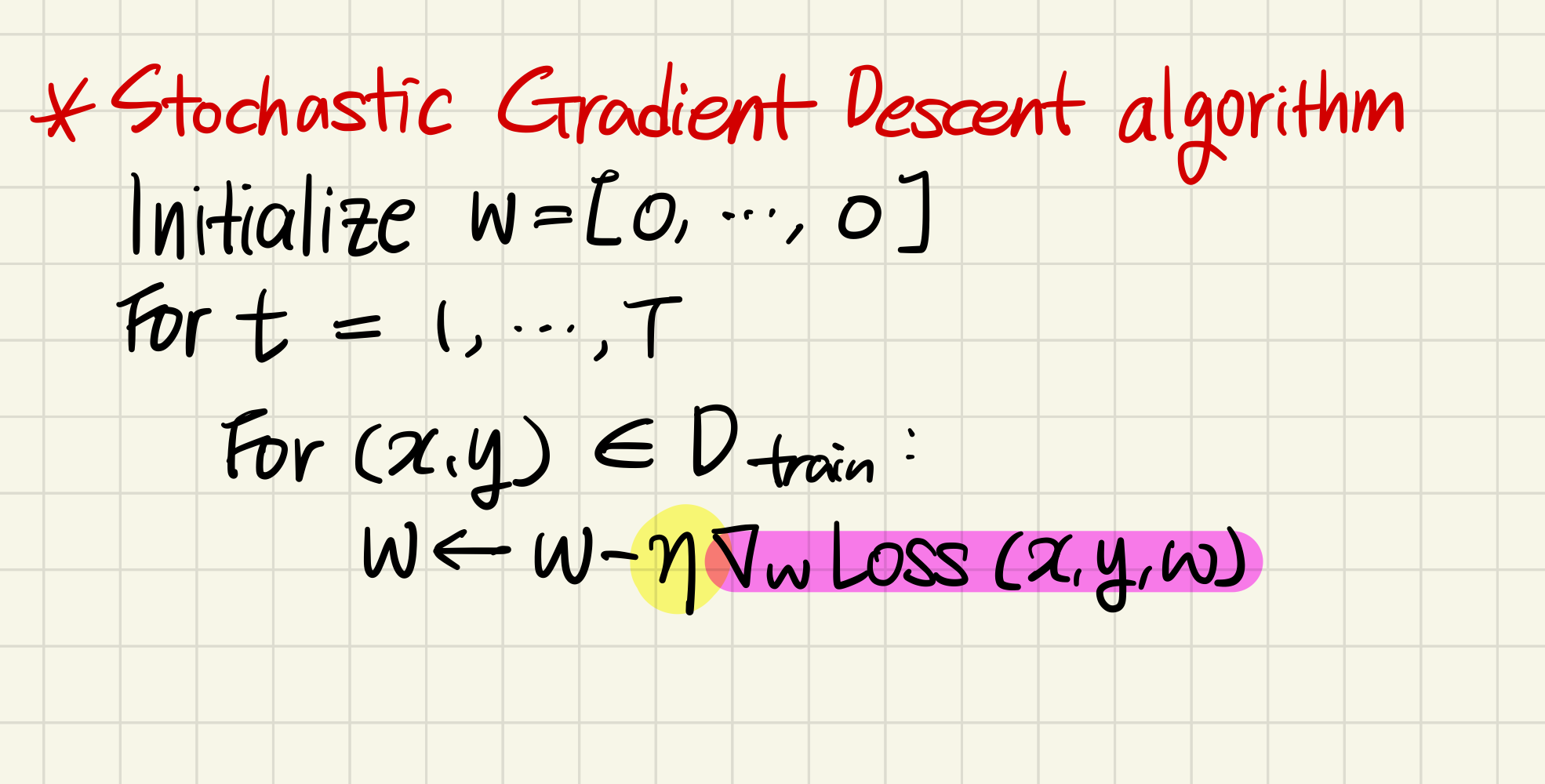
going through the training set, and after each example, make an update

 

it is faster in terms of having the number of updates be large.

 

 

 

* Step Size

update includes a step size η

it determines how far in the direction of the gradient or away from the gradient do you want to move

 

what should eta be?

possible range of eta: 0 ~ 1

0: conservative, more stable, less likely to bounce around

1: more aggressive step, move faster, perhaps at the risk of being more unstable

 

typical strategies choosing a step size

(1) just use constant step size: ex) η = 0.1

(2) use deacreasing step size rate: ex) η = 1 / the number of updates made so far

intuition of strategy (2) : as soon as tou start getting close to the optimum, it will slow down

 

Artificial Intelligence and Machine Learning 5 - Group DRO | Stanford CS221: AI (Autumn 2021)

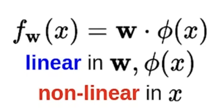
issue) fitting a non-linear predictor

 

it allows us to get non-linear predictors using the machinary of a linear predictor

 

Artificial Intelligence & Machine Learning 7 - Feature Templates | Stanford CS221: AI (Autumn 2021)

1. feature extraction with feature

example task:

string (x) → $f_{\omega}(x) = sign(\omega \cdot \phi(x))$ → valid email address?

question:

what properties of x might be relevant for predicting y?

feature extractor:

given x, produce set of (feature name, feature value) pair

2. prediction with feature names

score: weighted combination of features

$\omega\cdot\phi(x) = \sum_{j=1}^{d}\omega_{j}\phi(x)_j$

result : -1.2(1) + 0.6(0.85) + 3(1) + 2.2(1) + 1.4(0) = 4.51

 

if $\phi(x)_j$ is 1, and if $w_j$ is also positive,

it means it's voting in favor of positive classification

the magnitude of $w_j$ determines the strength of the vote

 

3. how do we choose these feature vectors?

which features to include? need an organizational principle

more systematic way == feature templates

 

4. feature template

definition: a group of features all computed in a similar way

define types of pattern to look for, not particular patterns

example : abc@gmail.com

[Feature template]	[Example feature]
last three characters equals ____	last three characters equals com    :   1
length greater than ____	length greater than 10    :   1
fraction of alphanumeric characters	fraction of alphanumeric characters    :   0.85

 

5. two feature vector implementations

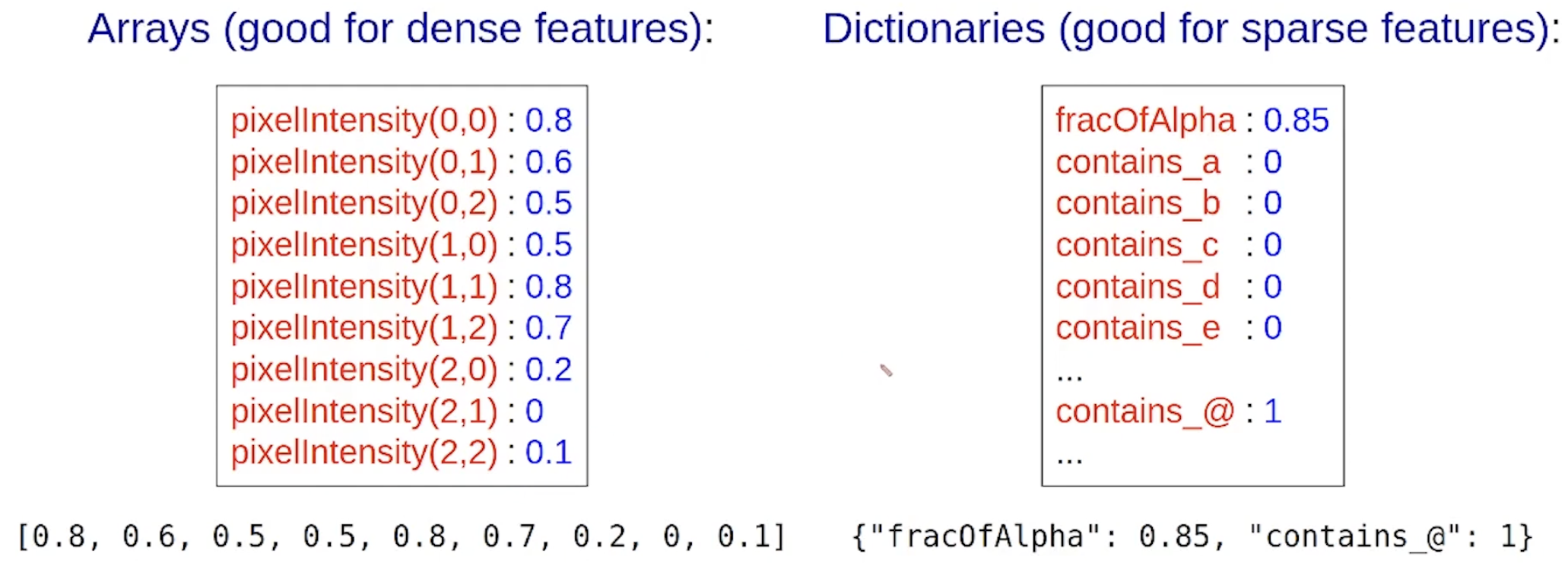
(1) arrays : good for dense features

(2) dictionaries : good for sparse features

 

 

Artificial Intelligence & Machine Learning 8 - Neural Networks | Stanford CS221: AI (Autumn 2021)

 

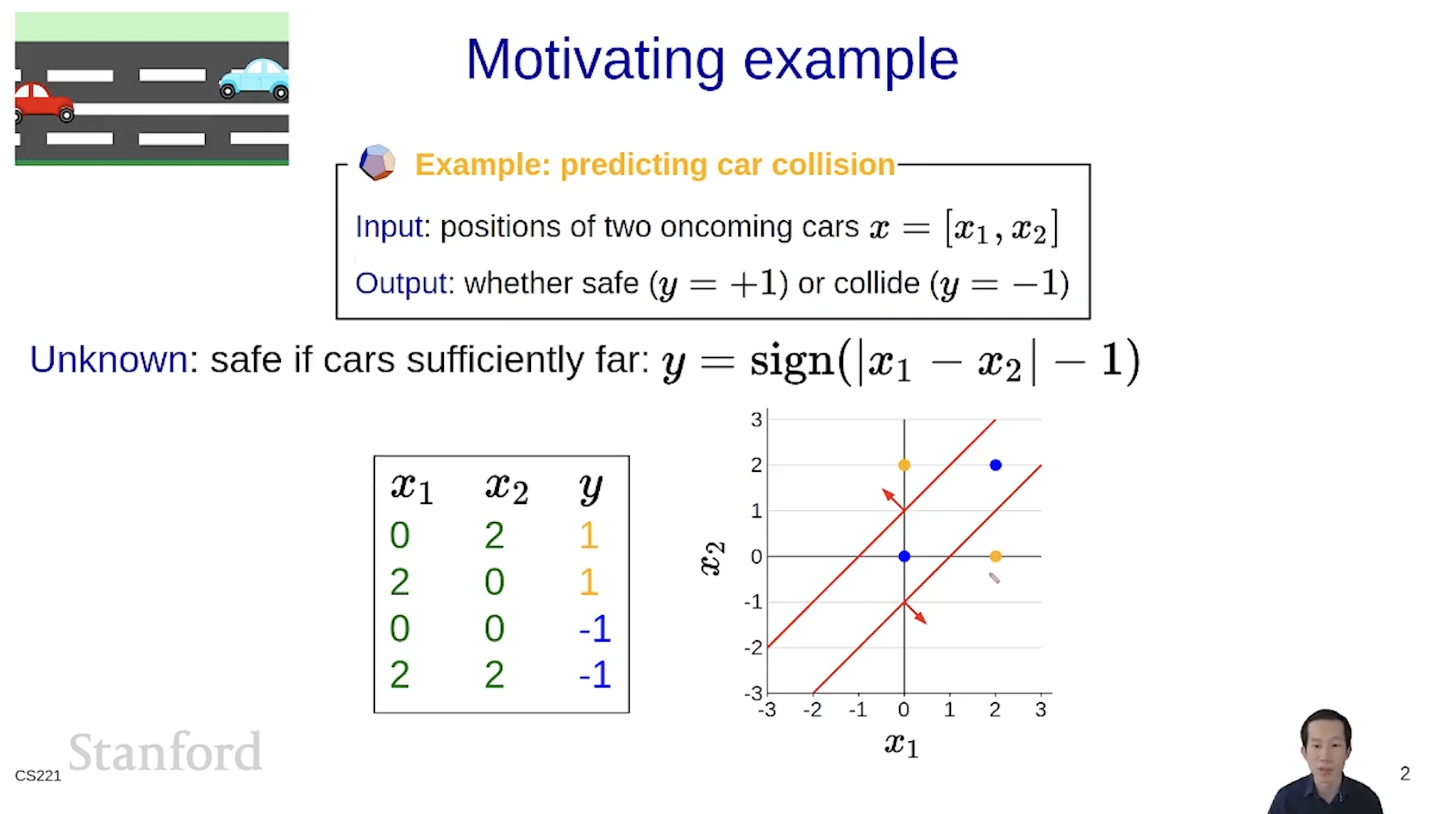
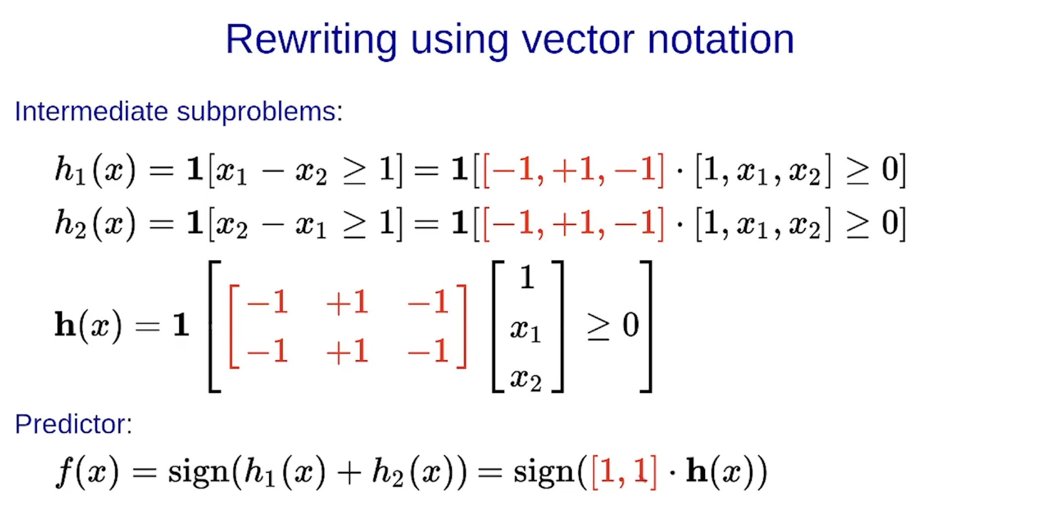
(1) key intution : the idea of problem decomposition

zero-one loss는 gradient가 zero가 된다는 특성 때문에 gradient descent, stochastic gradient descent를 사용하지 못한다는 단점이 있었음.

 

(2) avoid zero gradients

어우 질렸음 9분부터 다시 듣겠습니다